Lab 2, Ioan Dragomir

Exercise 1: bouncing ball

Simulate the bouncing ball demo available in Matlab and look at the functionality of each block. Create a new mdl file and rebuild the bouncing ball model.

I will skip over the first part, go and take a look for yourself! Let's build it from scratch!

We may start with the mathematical model in the form of a couple of differential equations...

\[ \begin{cases} \frac{dy}{dt} = v \\ \frac{dv}{dt} = -g \\ \text{when } y \leq 0,\quad v \gets | v | \end{cases} \]

...and just place integrators for each 1DE and a condition on \( y \) to reset \( v \), but that way we might miss the essence of what we are actually telling simulink to do. Thus, I will also provide a hopefully intuitive build up to these sstructures.

Integrators - how do we use them?

The integrator block is one of the most useful blocks in simulating physical systems. We will use integrators whenever we want to continuously change some value and we know how to compute "by how much" it changes at each step. Mathematically, this is equivalent to solving an ODE: the result of the integrator is the integrated value, and the input is the value of the differential.

\( \frac{dy}{dt} = [\cdots\text{ integrator gets this as input }\cdots]\)

And it outputs an approximation of \( y \).

It is important, though, to understand that it doesn't "compute the integral" in the way we would do when solving a math problem. It doesn't magically find "the formula of the result" from the beginning. (expect when it figures out it's a very easy math problem) It calculates the "current value" of the integral live, progressively, as more input data comes in, by adding it up. Like a Riemann sum, but a dumb Riemann sum that only knows values from the past and tries to predict the future. It doesn't have any clue about the overall behaviour of the system.

Check out lab2_extra.html for more info on how integrators work!

The falling ball

To simulate the falling ball, we must first think about what influences what. In our case, the position changes directly according to the velocity, and the velocity changes directly according to the acceleration, which is just the one due to gravity.

In simulink, we can represent this using two integrators:

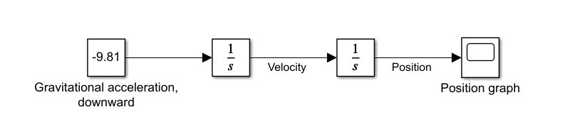
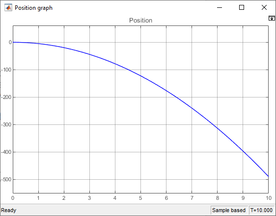
In this simulation, at each time step the first integrator will add \( -9.81 \cdot \Delta t \) to its output, thus obtaining the velocity \( v \) at that time, and the second integrator will add \( v \cdot \Delta t \) to its output, thus changing the position in concordance with the current speed. Note, again, that they do not know the whole speed/position functions from the start, but rather they "discover" the speed and position values, time step by time step.

Initial conditions

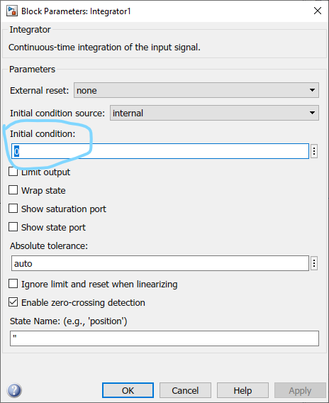
By default, all integrators start at 0. This means that our simulation supposes the ball starts at position 0 and velocity 0. If we want to change that, we may set the initial values inside the integrator's properties:

Or we can choose to set the initial value from the data flow graph, by selecting "Initial condition source: external", which will make the block now accept another input:

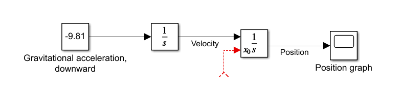
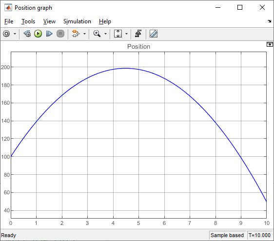
Connecting some value to this input will force the integrator to start with that value. For example, here's what happens if we start at position 100 and speed 44:

Making the ball bounce

We may also add a third input, an "external reset", which may tell the integrator, at any time, to start all over and grab a new "initial value", even if it's the middle of the simulation. We will use this functionality to implement the ball bounce, where the velocity needs to abruptly change in a way slightly hard to describe using just differential equations.

When the ball hits the ground, i.e. position <= 0, we want to suddenly set the velocity to point upwards, and lose a bit of momentum. (coefficient of restitution)

We can achieve this with the following model:

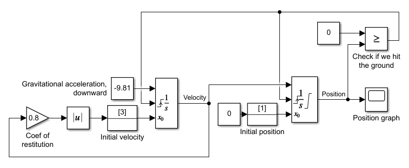
We now have a block to check when we hit the ground (top right), case in which it signals both the position and velocity integrators to reset (through the top signal line): something's up! When this happens, we reset the position to 0 and velocity to \( | 0.8 \cdot v_{prev} | \). The "Initial condition" blocks are there to differentiate between resetting the integrators at the beginning of the simulation, when we want to give them the initial values, and resetting them when the ball bounces.

We can see the graph looks like a bouncing ball :D

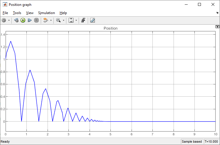
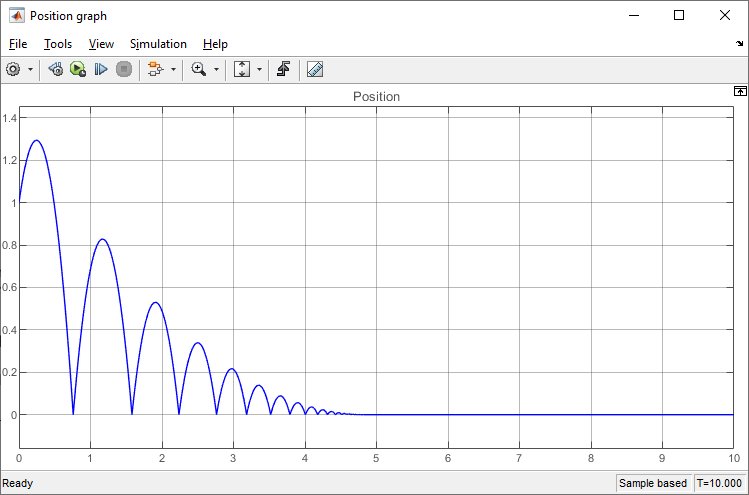
We can notice, though, that the temporal resolution is rather lacking, and the graph looks "jagged". Because matlab notices the system can be put into analytic form, (by clever use of symbolic solvers) it does that for us and only evaluates it at a handful of points. It doesn't need to evaluate anything other than the discontinuities when the ball bounces, but also is nice and shows us the peaks. We may reconfigure this by going into the model settings (Ctrl-E) > Solver > Solver details, and setting the "Max step size" to something smaller, like 0.01:

Download bouncing ball mdl!

Exercise 2: simple pendulum

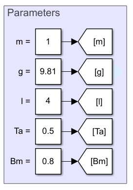
Simulate the model for the simple pendulum with the following parameters:

\( l=4,\,g=9.81,\,B_m=8,\,m=1 \), maximum step for the numerical simulation of 0.1 and the applied torque represented through a triangular signal with amplitude 1 and frequency of 0.1rad/sec.

Once again, we have a second order differential equation, but this time relating various torques to the angular velocity and thus angular position of the pendulum.

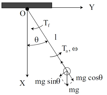
\( J = \text{"moment of intertia w.r.t. the pivot"} = ml^2 \)

\( T_a = \text{"torque applied externally"} \)

\( T_f = \text{"torque due to friction"} = B_m \cdot \omega /J = \frac{B_m\omega}{ml^2} \)

\( T_g = \text{"torque due to gravity"} = mgl\sin\theta /J = \frac{g\sin\theta}{l} \)

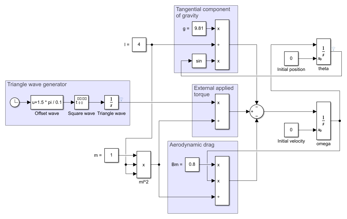
A design decision I took was to use Goto/From blocks for signal routing. It is the difference between this rat's nest...

...and this slightly more readable system...

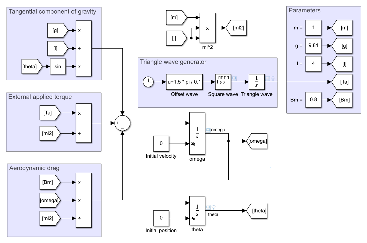
...the main difference being that we have less intertwined signal lines and more labeled inputs. It makes it both easier to read and less error-prone.

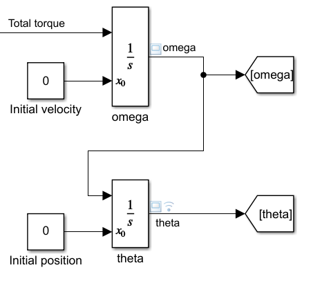
In any case, we may start by building the double integrator that will process a torque into an angular velocity \(\omega\), and that into an angular position \(\theta\):

Then compute the torque from both the parameters...

...and the state variables, in three parts which are all added up with the correct sign...

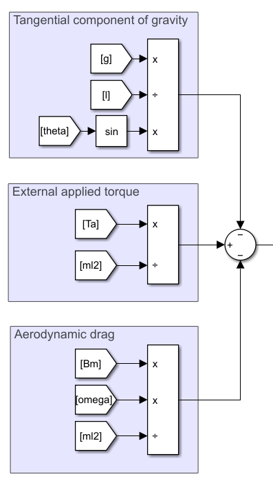
...and fed into the integrators we built earlier.

Triangle wave generation

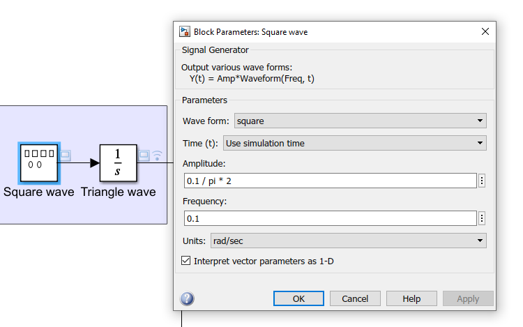
Lastly, we need to generate a triangle wave of given amplitude and frequency. It seems simulink doesn't have a block capable of directly doing that, so we must build it separately.

A triangle wave is the integral of a square wave centered around 0. For each high or low section of the square wave with amplitude \(A\) and half-period \(T/2\), the triangle wave changes by \(\pm A \cdot T/2\). The square wave's period must match that of the triangle wave, so we may only control its amplitude and phase:

\( T = \frac{2\pi}{0.1rad/s} = 20\pi s \)

\( A_{triangle} = 1/2 \cdot A_{square} \cdot T/2 = 1\quad \Rightarrow A_{square} = \frac{1}{5\pi} \)

We may generate a square wave with the given amplitude and period by use of a Signal Generator block:

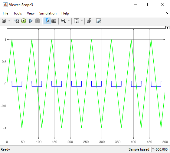
Now the only issue might be that the square wave starts on a negative half-period, and thus the triangle wave starts by going down from 0 to -2:

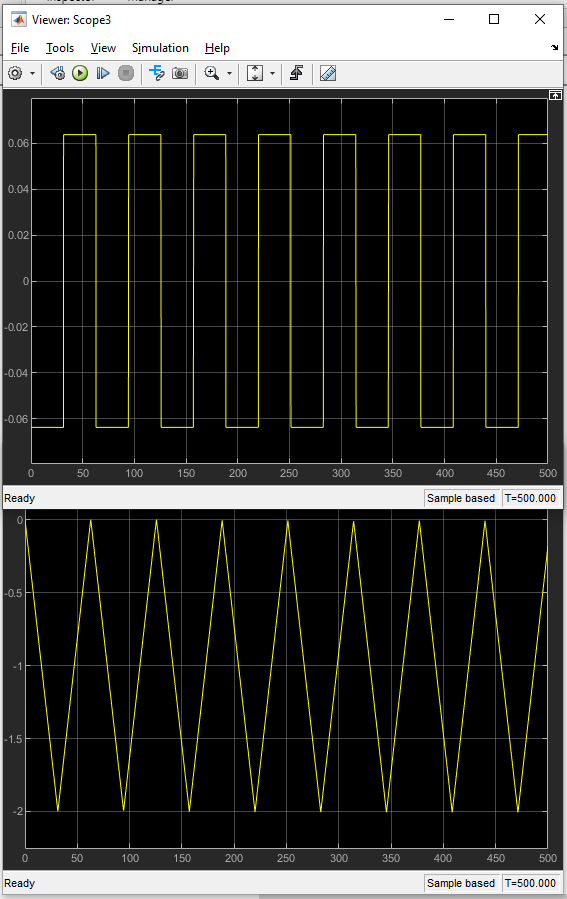
I would prefer the triangle wave to start from 0 and rise to 1, then go back down, so I would need to shift the square wave to start at its last quarter-wavelength...

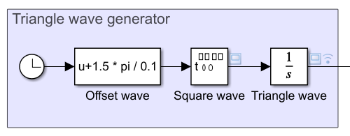
...leading to this waveform...

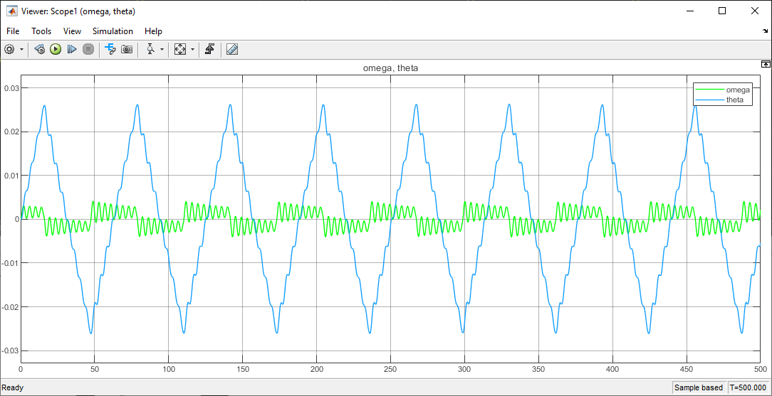
...and this final pendulum swing graph:

Download pendulum mdl!

Extra eye candy

While we're at it, why not use the data from our simulations to also graphically display what's going on? While I tried to use MATLAB's builtin animation and plotting facilities, I found them rather clunky and hard to use, so I resorted to HTML5 animations. If you're reading the PDF, go check them out on https://trupples.space/uni/2/ProcessModeling/html/lab2.html!