Lab 2 extras: How do integrators work?
You can skip this section if you think you have a good enough intuition of how Riemann sum integrals relate to changes in the physical world.
In the real world we can consider processes perfectly continuous (this sparks a very intriguing debate on how continuous physical processes really are, hehe planck time, hehe time dillation, hehe paradoxes, get me drunk and I'll spend a night on this) But when simulating such processes, if we can't describe them fully analytically, (i.e. we can't find a formula that will exactly predict its behaviour; in this case we can, but we will pretend we can't) we will have to resort to "approximating" the time continuity using very tiny time steps.
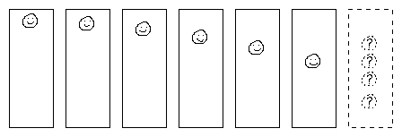
A movie captures a continuous process as a series of quick frames. The more frames per unit time, the smoother the movie is. If we had a movie of a falling ball and it suddenly stopped, we could predict where the ball would be in the next frames (our brain does that automatically, but I mean on paper), but we are limited by the resolution of the movie, especially the temporal resolution. If our frames are spaced wide apart in time, we have a greater risk of accumulating errors due to the system not being linear. If our frames are closer in time, we will have smaller errors (we can better approximate small bits of the signal by linear functions, lest we have to deal with fractal-like behaviour) but it will take more steps and computing power to simulate.

If we take very small steps in time, let's say \( 1/100 \) of a second, we'll see that the acceleration "adds to" the speed \( g/100 \), and the speed "adds to" the position roughly \( v/100 \). (Mathematically, this corresponds to \( \frac{dv}{dt} = g \) and \( \frac{dx}{dt} = v \)) The second one isn't exact, though, because the speed isn't constant over this time interval, but it will be close. Repeat this for many time slices of \( 1/100\, s \) and we can simulate the dynamics of a ball that's falling and picking up speed.
There are more complicated algorithms we will learn in the Numerical Calculus course to minimize such errors, but the gist of it is that if we keep on accumulating these small changes (i.e. derivatives) to a variable, it will approximate the integral of those small changes.
This is what the integrator block does! For each time step, it takes in a "small change" as an input, and adds it to its result. If we input acceleration data, it will output speed by adding up the acceleration over multiple time steps. If we input speed, it will output position. If we input daily earnings, it will output our bank balance.
Notice, though, how it doesn't represent the integral as a known and exactly computable function, the way we do in analysis, but it emulates the process of integration by adding up derivatives.