Lab 3, Ioan Dragomir

Intro

Symbolic variables may be used to implement various mathematical constructions and relations without actually computing values at each step.

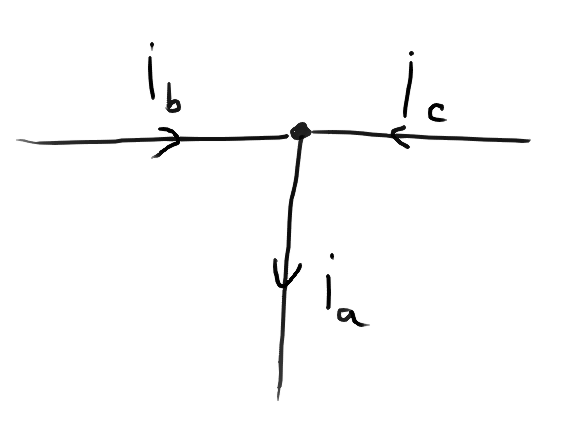
For example, in an electrical circuit, it is not the same to say that mathematically \( I_a = I_b + I_c \) and programatically \( I_a \gets I_b + I_c \). The latter obtains \( I_a \) given \( I_b \) and \( I_c \), while the first is a relation that might be rearranged to obtain other formulas.

The symbolic toolbox allows us to declare such symbolic variables and operate on them in such a way that relations between them are preserved.

Differentiation

The diff function may be used to compute the differential of an expression. Here we can further see the distinction between symbolic and non-symbolic operations. When operating with symbolic variables, the differentials are what we would mathematically expect:

syms x;
disp("Differential of a symbolic expression x^3: ")
x^3
diff(x^3)

Differential of a symbolic expression x^3: 
ans =
x^3
ans =
3*x^2

When operating with a non-symbolic variable, though, all calculations are performed to obtain a constant number, which is then passed to diff, but the differential of a constant is null, so we don't get the answer we might expect:

t = 10;
disp("Differential of a non-symbolic expression t^3: ")
t^3
diff(t^3)

clear t;

Differential of a non-symbolic expression t^3: 
ans =
        1000
ans =
     []

We may also take differentials of functions. diff also takes an optional second parameter to specify the derivative order:

syms x;
f = @(x)(x^3 + x^2 - 3*x);
disp("1st, 2nd, and 3rd order differentials of f: ")
f
diff(f(x))
diff(f(x), 2)
diff(f(x), 3)

1st, 2nd, and 3rd order differentials of f: 
f =
  function_handle with value:
    @(x)(x^3+x^2-3*x)
ans =
3*x^2 + 2*x - 3
ans =
6*x + 2
ans =
6

Partial derivatives

Another optional parameter of diff may specify which variable to differentiate by. For example, here's how we can calculate

\[ \frac{d}{dx} x^3y = 3x^2y \\ \frac{d}{dy} x^3y = x^3 \]

syms x y;
f = x^3 * y
diff(f, x)
diff(f, y)

f =
x^3*y
ans =
3*x^2*y
ans =
x^3

If no variable is provided, matlab chooses one by some internal criteria. We may query which variables it considers most relevant in this sense by use of the symvar function (previously known as findsym):

syms x y z;
F = x * (x * y + y * z);

symvar(F, 1)

ans =
x

Solving differential equations

A very useful feature is the dsolve function, which receives some symbolic relations, often involving differentials, (i.e. a system of differential equations) and computes a solution.

Say we would like to solve the following system:

\[ \begin{cases} \frac{dy}{dt} = z \\ \frac{dz}{dt} = -y \\ y(0) = 3 \\ z(0) = 1 \end{cases} \]

We will need to write 4 such "symbolic conditions" for each of the relations described above, and pass them all to dsolve.

First, it is important that y and z are functions of time, not just some ordinary single-value variables:

syms t y(t) z(t);

Then, we may write each of the differential equations like so:

eq1 = diff(y, t) == z;
eq2 = diff(z, t) == -y;

And the initial conditions like so:

ic1 = y(0) == 3;
ic2 = z(0) == 1;

And use dsolve to compute a solution to the system, passing it a vector of equations and a vector of initial conditions:

solution = dsolve([eq1, eq2], [ic1, ic2])

solution = 
  struct with fields:

    z: cos(t) - 3*sin(t)
    y: 3*cos(t) + sin(t)

We could have also just provided the expressions directly to dsolve to get the same result:

solution2 = dsolve(...
    [ ... % First comes the system of equations
        diff(y, t) == z, ...
        diff(z, t) == -y ...
    ], ...
    [ ... % And then a system of initial conditions
        y(0) == 3, ...
        z(0) == 1 ...
    ] ...
)

solution2 = 
  struct with fields:

    z: cos(t) - 3*sin(t)
    y: 3*cos(t) + sin(t)

Integration

On the other hand, we may compute integrals of symbolic functions using int.

For example, to compute

\[ \int_{-3}^{44} x^3 \cdot \arctan(x)\,dx = ??? \]

We may write:

syms x;
int(x^3 * atan(x), x, -3, 44)

ans =
20*atan(3) + (3748095*atan(44))/4 - 42535/6

Limits

Another calculus operation we can do on symbolic variables is the limit, using limit.

For example,

\[ \lim_{x\to\infty} \left(1+\frac{1}{x} \right)^{x} = e \]

May be computed like so:

syms x;
limit((1 + 1/x)^x, x, inf)

ans =
exp(1)

Sums and products

While the functions sum and prod may calculate sums and products of non-symbolic variables with actual concrete values, symsum and symprod can deduce more abstract sums involving symbolics:

\[ A = \sum_{k=a}^{b} k^2 = ??? \] \[ B = \prod_{k=a}^{b} \frac{1}{k} = ??? \]

syms k a b;
A = symsum(k^2, k, a, b)
B = symprod(1/k, k, a, b)

A =
(b*(2*b + 1)*(b + 1))/6 - (a*(2*a - 1)*(a - 1))/6
B =
piecewise(1 <= a, factorial(a - 1)/factorial(b), b <= -1, ((-1)^(b + 1)*factorial(- b - 1))/((-1)^a*factorial(-a)))

Substitution

Given a symbolic expression, say \( 3x+y^4 \), we may want to actually start replacing some of the variables with values, let's say \(x = 3\). To do this, we use the subs function:

syms x y;
f = 3*x + y^4;
subs(f, x, 3)

ans =
y^4 + 9

If by substitution we get to a constant, we need to keep in mind it's still a symbolic object, so any operations with it will keep its "symbolic-ness". To get around this, we may convert it to a double or an int:

syms x;
f = 3*(x+1)*(x-1);

y = subs(f, x, 12);

y
type_of_y = class(y)
y_plus_13 = y + 13
type_of_y_plus_13 = class(y + 13)

y_converted = double(y)
type_of_y_converted = class(y_converted)
y_converted_plus_13 = y_converted + 13
type_of_y_converted_plus_13 = class(y_converted + 13)

y =
429
type_of_y =
    'sym'
y_plus_13 =
442
type_of_y_plus_13 =
    'sym'
y_converted =
   429
type_of_y_converted =
    'double'
y_converted_plus_13 =
   442
type_of_y_converted_plus_13 =
    'double'

We may also substitute by other symbolic values, not necessarily constants:

syms x y t;
f = cos(x) * y;

subs(f, x, acos(t)) % replace x with arccos(t)

ans =
t*y

Or even replace whole parts of the expression:

syms x y t;
f = cos(x) * y;

subs(f, cos(x), y^3) % replace cos(x) with y^3

ans =
y^4

Simplifying, expanding, factoring

There is a collection of functions capable of doing basic algebraic manipulation on symbolic expressions, such as taking a common factor, simplifying, and expanding products.

expand, factor

As their names suggest, expand takes an expression and "expands" all products of parantheses to sums of products of individual terms, and factor tries to take out common factors.

\[ (x^2 + 3)(x - 5) = x^3 - 5x^2 + 3x - 15 \]

syms x;
expand((x^2 + 3) * (x - 5))
factor(x^3 - 5*x^2 + 3*x - 15)

ans =
x^3 - 5*x^2 + 3*x - 15
ans =
[x - 5, x^2 + 3]

collect

collect rearranges the expression in the form of a polynomial of a given variable. For instance, we may rewrite

\[ F = \cos(a) \cdot x^3 + (x^2 - 1)(y + x - 3) \]

as a polynomial in \(x\) as

\[ F = (\cos(a) + 1)x^3 + (y - 3)x^2 - x - y + 3 \]

or as a polynomial in \(y\) as

\[ F = (x^2 - 1)y + (x^2 - 1)(x - 3) + x^3\cos(a) \]

syms a x y;
collect(cos(a) * x^3 + (x^2 - 1) * (y + x - 3), x)
collect(cos(a) * x^3 + (x^2 - 1) * (y + x - 3), y)

ans =
(cos(a) + 1)*x^3 + (y - 3)*x^2 - x - y + 3
ans =
(x^2 - 1)*y + (x^2 - 1)*(x - 3) + x^3*cos(a)

horner

horner rearranges the polynomial according to Horner's rule:

\[ \begin{aligned} a_0 &+ a_1x + a_2x^2 + a_3x^3 + \cdots + a_nx^n \\ &= a_0 + x \bigg(a_1 + x \Big(a_2 + x \big(a_3 + \cdots + x(a_{n-1} + x \, a_n) \cdots \big) \Big) \bigg) \end{aligned} \]

For instance, \( 4x^5 - 2x^4 + 8x^3 - x + 5 = x(x(x(x(4x - 2) + 8) + 0) - 1) + 5\)

syms x;
horner(4 * x^5 - 2 * x^4 + 8 * x^3 - x + 5)

ans =
x*(x^2*(x*(4*x - 2) + 8) - 1) + 5

simplify

simplify tries to manipulate an expression to bring it to a simpler form. For example:

\[ \frac{e^{jx} + e^{-jx}}{2} = \cos(x) \]

\[ x\cdot x\cdot x\cdot x = x^4 \]

simplify((exp(1j*x) + exp(-1j*x))/2)

simplify(x * x * x * x)

ans =
cos(x)
ans =
x^4

Exercise 1 - differentials

Differentiate the following functions:

\[ f(x) = \arcsin(2x+3) \]

syms x;
diff(asin(2 * x + 3))

ans =
2/(1 - (2*x + 3)^2)^(1/2)

\[ f(x) = arctan(x^2 + 1) \]

syms x;
diff(atan(x^2 + 1))

ans =
(2*x)/((x^2 + 1)^2 + 1)

Exercise 2 - integrals

Calculate the following integrals:

\[ \int x\sin(x^2) dx \]

syms x;
int(x * sin(x^2))

ans =
-cos(x^2)/2

\[ \int x^2 \sqrt{x + 4} \]

syms x;
int(x^2 * sqrt(x + 4))

ans =
-(2*(x + 4)^(3/2)*(168*x - 15*(x + 4)^2 + 112))/105

\[ \int_{-\infty}^{\infty} e^{-x^2} dx \]

syms x;
int(exp(-x^2), -inf, inf)

ans =
pi^(1/2)

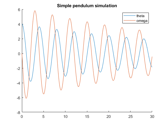
Exercise 3 - simple pendulum

We are required to use the small angle approximation that \( x \approx \sin(x) \). Otherwise, the symbolic solver will not find a solution and the code won't work.

We start by declaring pos and vel to be symbolic functions in time and setting some parameters:

syms pos(t) vel(t);

Bm = 0.8;
m = 1;
l = 4;
g = 9.81;

Then we provide these differential equations:

\[ \begin{cases} \frac{d\theta}{dt} = \omega \\ \frac{d\omega}{dt} = \frac{-B_m}{ml^2}\omega - \frac{g}{l}\theta \end{cases} \]

and these initial conditions:

\[ \begin{cases} \theta(0) = 4 \\ \omega(0) = 0 \end{cases} \]

to dsolve:

pendulum_sol = dsolve([ ...
    diff(pos) == vel, ...
    diff(vel) == -Bm/(m*l^2) * vel - g/l * pos...
],[ ...
    pos(0) == 4, ...
    vel(0) == 0 ...
]);

pendulum_sol, the object returned by dsolve, contains multiple fields corresponding to the solutions for the unknown variables. We extract the position and velocity functions from the solution object and plot them:

theta = pendulum_sol.pos;
omega = pendulum_sol.vel;

clf;
hold on;
fplot(theta, [0, 30]);
fplot(omega, [0, 30]);
title("Simple pendulum simulation");
legend(["theta", "omega"]);

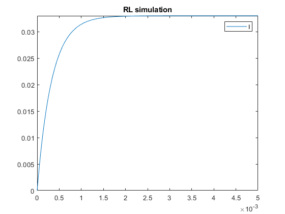
Exercise 4 - RL circuit

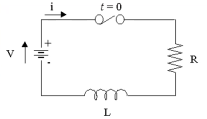
Similarly to lab 1, ex 3, we may write the whole differential equation like so:

\[ Ri + L\frac{di}{dt} = V \]

This can be implemented like:

syms I(t);

R = 100;
V = 3.3;
L = 33e-3;

circuit_solution = dsolve(R * I + L * diff(I) == V, I(0) == 0);
% Note: since only one symbolic variable appears in the system, dsolve
% deduces that's what we want to solve for and only returns a function,
% unlike the previous case where it returned a structure with multiple
% functions, one for each symbolic variable.

clf;
fplot(circuit_solution, [0, 5e-3]);
title("RL simulation");
legend("I");

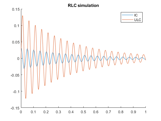
Exercise 5 - RLC circuit

Consider that the RL electrical circuit from the previous example is augmented by adding a \(2000 \mu F\) capacitor in parallel with the inductor. Use the symbolic toolbox for building the dynamic model and simulate the voltage across and the current through the capacitor, using the following values of the other paramerets: \( R = 100\Omega,\,V=3.3V,\,L=33mH \).

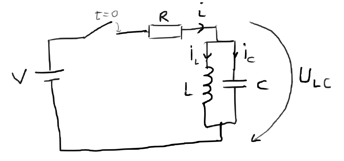
\[ \begin{cases} i = i_L + i_C \text{\quad by KCL}\\ U_{LC} = L\frac{di_L}{dt} \text{\quad by the inductor formula}\\ i_C = C\frac{dU_{LC}}{dt} \text{\quad by the capacitor formula}\\ V = iR + U_{LC} \text{\quad by KVL} \end{cases} \]

Here we have 3 variables (\(i_L,\,i_C,\,U_{LC}\)) but only 2 are independent (because of the first and last equations above, knowing any 2 of them will uniquely determine the third). If we provide all equations, dsolve will complain that there are more equations than independent variables. It tries to reduce the number of equations, but in this case it fails, so we hve to assist it. We have to reduce the system down to 2 differential equations and 2 initial conditions. I chose \(i_L\) and \(U_{LC}\), so I need to rewrite \(i_C = i - i_L = (V-U_{LC})/R - i_L\):

\[ \begin{cases} \frac{di_L}{dt} = \frac{U_{LC}}{L} \\ \frac{dU_{LC}}{dt} = \frac{1}{C}\left(\frac{V-U_{LC}}{R} - i_L\right) \\ U_{LC}(0) = 0 \\ i_L(0) = 0 \end{cases} \]

syms il(t) ulc(t);

R = 100;
V = 3.3;
L = 33e-3;
C = 2000e-6;

circuit_sol = dsolve([ ...
    diff(il) == ulc / L, ...
    diff(ulc) == ((V - ulc) / R - il) / C, ...
], [ ...
    ulc(0) == 0, ...
    il(0) == 0 ...
]);

il_sol = circuit_sol.il;
ulc_sol = circuit_sol.ulc;
ic_sol = ((V - ulc_sol) / R - il_sol);

clf;
hold on;
fplot(ic_sol, [0, 1]);
fplot(ulc_sol, [0, 1]);
title("RLC simulation");
legend(["IC", "ULC"]);