Lab 1 homework, Ioan Dragomir

Overview of called functions:

plot_ex1_1;
plot_ex1_2;
plot_ex1_3;
check_ex2;
plot_ex3;

Exercise 1

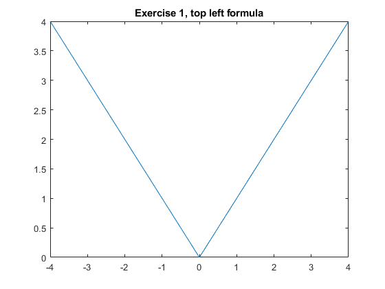
Write functions to plot the following signals:

1. \( y = \begin{cases} -t, &t \in [-4, 0) \\ t, &t \in [0, 4] \end{cases} \)

function y = ex1_1(t)
    if t >= -4 && t < 0
        y = -t;
    elseif (t >= 0 && t <= 4)
        y = t;
    end
end

function plot_ex1_1
    t = -4 : 0.01 : 4;
    y = arrayfun(@(x) ex1_1(x), t); % What awful syntax... Can't I just
                                    % declare that the function takes in a
                                    % scalar and have it automagically
                                    % vectorize ex1_1(t) for me, as it does
                                    % in, say, sin(t)? Or must each
                                    % function implement this internally
                                    % and sin() has this arrayfun logic
                                    % applied after entering the function,
                                    % not by the language beforehand?
    plot(t, y);
    title("Exercise 1, top left formula");
end

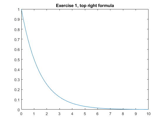
2. \( y = 0.5^t,\quad t \in [0, 10] \)

function y = ex1_2(t)
    if t >= 0 && t <= 10
        y = 0.5^t;
    end
end

function plot_ex1_2
    t = 0 : 0.01 : 10;
    y = arrayfun(@(x) ex1_2(x), t);
    plot(t, y);
    title("Exercise 1, top right formula");
end

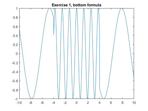
3. \( y = \begin{cases} \sin(t), &\{-10 \leq t \le 4\} \cup \{4 \le t \le 10\} \\ \cos(5t), &-4 \le t < 4 \end{cases} \)

function y = ex1_3(t)
    if (t >= -10 && t < -4) || (t >= 4 && t <= 10)
        y = sin(t);
    elseif t >= -4 && t < 4
        y = cos(5*t);
    end
end

function plot_ex1_3
    t = -10 : 0.01 : 10;
    y = arrayfun(@(x) ex1_3(x), t);
    plot(t, y);
    title("Exercise 1, bottom formula");
end

Exercise 2

Write a function for computing the factorial of a number n ( \( n! \) )

function nf = factorial(n)
    nf = 1;
    for i = 1:n
        nf = nf * i;
    end
end

function check_ex2
    assert(factorial(1) == 1)
    assert(factorial(3) == 6)
    assert(factorial(5) == 120)

    disp("No assert errors => Factorials are OK!");
end

No assert errors => Factorials are OK!

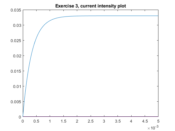
Exercise 3

Consider a model for an electric circuit which contains a resistor, an inductor, a continuous voltage source and a switch, in series.

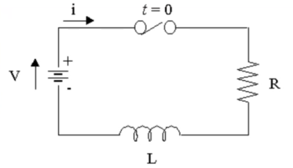
If at time \( t = 0 \) the switch is turned on (prior to this moment the current in the inductor is zero), the following equation is valid:

\[ L \frac{di}{dt} + Ri = V \]

Show that the solution to this equation is:

\[ i = \frac{V}{R}(1-\exp(-Rt/L)) \]

My solution is as follows. First we rearrange the terms to get the usual Linear Differential Equation form (1), then follow through with the usual LDE trick of creating a differential of a product and integrating it (2, 3, 4), to get a non-differential equation which we can solve algebraically (5, 6, 7).

\[ \begin{align} \frac{di}{dt} + i \frac{R}{L} &= \frac{V}{L} &|& \cdot e^{\int \frac{R}{L} dt} = e^{\frac{Rt}{L}} \\ \frac{di}{dt} e^{\frac{Rt}{L}} + i \frac{R}{L} e^{\frac{Rt}{L}} &= \frac{V}{L} e^{\frac{Rt}{L}} &|& a'b + ab' = (ab)' \\ \frac{d}{dt}(i \cdot e^{\frac{Rt}{L}}) &= \frac{V}{L} e^{\frac{Rt}{L}} &|& \int \ldots dt \\ \int\frac{d}{dt}(i \cdot e^{\frac{Rt}{L}}) dt &= \int \frac{V}{L} e^{\frac{Rt}{L}} dt && \\ i \cdot e^{\frac{Rt}{L}} &= \frac{V}{L} \cdot \frac{L}{R} e^{\frac{Rt}{L}} + C &|& \cdot e^{-\frac{Rt}{L}} \\ i &= \frac{V}{R} (e^{\frac{Rt}{L}} + C) e^{-\frac{Rt}{L}} && \\ i &= \frac{V}{R} (1 - C\cdot\exp(-Rt/L)) && \\ \end{align} \]

With this general form, we use the fact that \( t = 0 \Rightarrow i = 0 \) to get \( C = 1 \), thus confirming the solution for \( i(t) \):

\[ i = \frac{V}{R}(1-\exp(-Rt/L)) \]

function i = sim_circuit(t, V, L, R)
    i = V / R * (1 - exp(-R * t / L));
end

function plot_ex3
    V = 3.3;
    R = 100;
    L = 33e-3;
    t = 0 : 1e-5 : 5e-3;
    i = zeros(length(t)); % instead of [] so it won't complain abt resizing
    for ti = 1:length(t)
        i(ti) = sim_circuit(t(ti), V, L, R);
    end
    plot(t, i);
    title("Exercise 3, current intensity plot");
end