Lab 8, Ioan Dragomir

Computing integrals

Task: Compute the integral \(I = \int_0^{\pi/2}\sin x\,dx\).

We generate sequences of 10, 40, 80, and 10000 pseudorandom numbers in \([0; \pi/2]\), evaluate the function to be integrated at those points, and sum the results:

N = 10;
a = rand(1, N) * pi/2;
I10 = pi / (2*N) * sum(sin(a))

N = 40;
a = rand(1, N) * pi/2;
I40 = pi / (2*N) * sum(sin(a))

N = 80;
a = rand(1, N) * pi/2;
I80 = pi / (2*N) * sum(sin(a))

N = 10000;
a = rand(1, N) * pi/2;
I10000 = pi / (2*N) * sum(sin(a))

I10 =

    0.9557


I40 =

    0.8749


I80 =

    0.8502


I10000 =

    0.9988

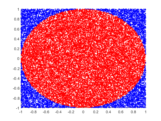
Approximating \(\pi\)

N = 30000;
points = rand(2, N) * 2 - 1;

is_inside = points(1,:) .^ 2 + points(2,:) .^ 2 <= 1;

clf;
hold on;
plot(points(1,is_inside), points(2,is_inside), 'r.')
plot(points(1,~is_inside), points(2,~is_inside), 'b.')

num_inside_circle = sum(is_inside);

pi_approx = 4 * num_inside_circle / N

pi_approx =

    3.1568

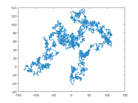
angles = rand(1, N) * pi - pi / 2;

walkx = zeros(1, N);
walky = zeros(1, N);

for i = 1:N-1
    r = floor(rand * 4);
    if r == 0
        walkx(i+1) = walkx(i) + 1;
        walky(i+1) = walky(i);
    elseif r == 1
        walkx(i+1) = walkx(i) - 1;
        walky(i+1) = walky(i);
    elseif r == 2
        walkx(i+1) = walkx(i);
        walky(i+1) = walky(i) + 1;
    else
        walkx(i+1) = walkx(i);
        walky(i+1) = walky(i) - 1;
    end
end

clf;
plot(walkx, walky)

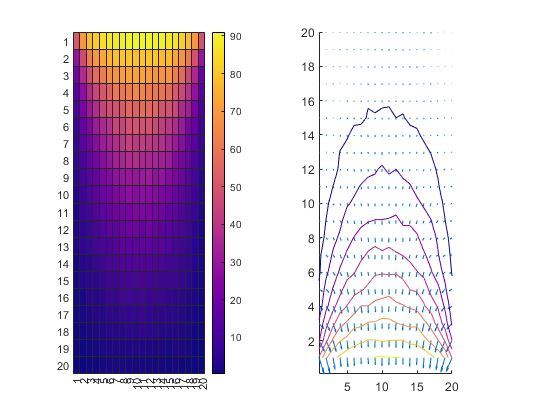
Using random walks to solve Laplace's equation

N = 1000000;

dim = 20;
potential = zeros(dim);
counts = zeros(dim);

for i = 1 : N
    x = floor(rand * dim + 1);
    y = floor(rand * dim + 1);
    xi = x; yi = y; % Save starting point
    while true
        r = floor(rand * 4);
        if r == 0
            x = x + 1;
        elseif r == 1
            x = x - 1;
        elseif r == 2
            y = y + 1;
        else
            y = y - 1;
        end

        if x == 0 || x == dim+1 || y == 0 || y == dim+1
            if x == 0
                potential_here = 100;
            else
                potential_here = 0;
            end
            potential(xi,yi) = potential(xi,yi) + potential_here;
            counts(xi,yi) = counts(xi,yi) + 1;
            break;
        end
    end
end

potential = potential ./ counts;

subplot(1, 2, 1);
heatmap(potential);
colormap('plasma');

subplot(1, 2, 2);
hold on;
[dx, dy] = gradient(potential);
quiver(dx, dy);
%[ex, ey] = gradient(potential);
contour(potential);
colormap('plasma');