Lab 6, Ioan Dragomir

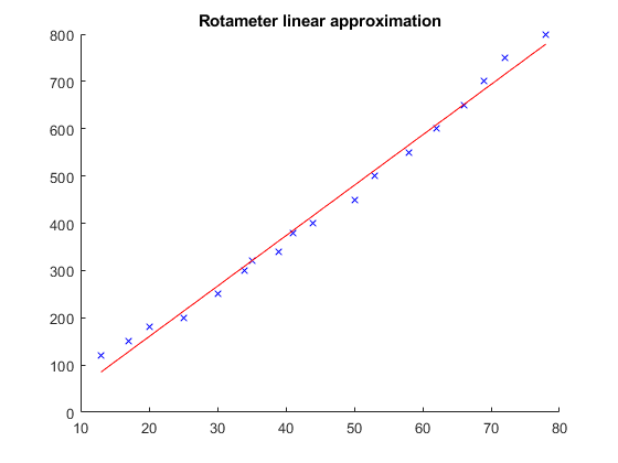
Exercise 1 - Rotameter calibration

flow_rate = [120; 150; 180; 200; 250; 300; 320; 340; 380; 400; 450; 500;
    550; 600; 650; 700; 750; 800];
height = [13; 17; 20; 25; 30; 34; 35; 39; 41; 44; 50; 53; 58; 62; 66; 69;
    72; 78];

f = fit(height, flow_rate, 'poly1')
c = coeffvalues(f);

a = c(1)
b = c(2)

clf;
hold on;
plot(height, flow_rate, 'bx');

x = xlim;

height_range = height(1) : height(end);
flow_estimated = height_range * a + b;

plot(height_range, flow_estimated, 'r-');
title("Rotameter linear approximation");

f = 

     Linear model Poly1:
     f(x) = p1*x + p2
     Coefficients (with 95% confidence bounds):
       p1 =       10.67  (10.14, 11.2)
       p2 =      -53.46  (-79.4, -27.52)

a =

   10.6728


b =

  -53.4604

We may also compute the means and standard deviations of the initial data set: (\(\bar q,\, \bar h,\, \sigma_q,\, \sigma_h\))

mean_q = mean(flow_rate)

mean_q =

  424.4444

mean_h = mean(height)

mean_h =

   44.7778

stddev_q = std(flow_rate)

stddev_q =

  213.0237

stddev_h = std(height)

stddev_h =

   19.8718

Exercise 2 - Modeling an alveola

We will model a lung alveola as an expandable compartment which is brought to a "closed" state by a spring. Air may escape through a tube, but it is restricted. We denote:

\[ \begin{aligned} \Delta P &= \text{ "pressure differential over the tube"} \\ P_{el} &= \text{ "elastic pressure"} \\ P &= \Delta P + P_{el} = \text{ "total pressure"} \\ V(t) &= \text{ "internal volume"} \\ V'(t) &= \text{ "flow rate"} \end{aligned} \]

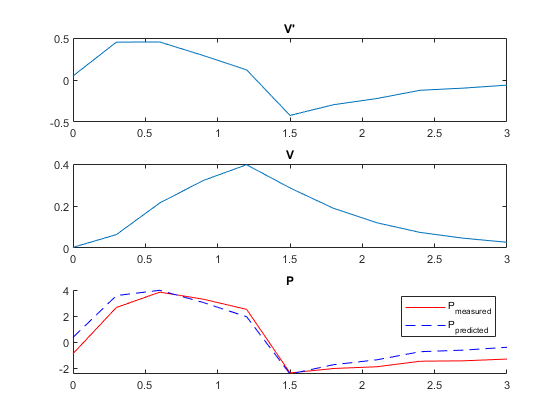
We have the following measured data for the flow rate \(V'\), internal volume \(V\) and total pressure \(\Delta P + P_{el} = P\) over a period of time:

t = [0; 0.3; 0.6; 0.9; 1.2; 1.5; 1.8; 2.1; 2.4; 2.7; 3];
dV_dt = [
    0.048; 0.4512; 0.4524; 0.2916; 0.1212; -0.4220; -0.2943; -0.2205; ...
    -0.1222; -0.0965; -0.0611
];
V = [
    0.0031; 0.0639; 0.2146; 0.3214; 0.3966; 0.2860; 0.1892; 0.1203; ...
    0.0741; 0.0465; 0.0273
];
P_measured = [
    -0.8796; 2.6633; 3.8347; 3.2975; 2.5159; -2.3584; -2.0160; -1.8821; ...
    -1.4588; -1.4265; -1.2926
];

We construct a model which predicts the total pressure depending on the volume and flow rate.

First, we consider the alveola's elasticicity to obey Hooke's law, and thus the elastic force should be proportional to the total "displacement" of the spring, which is proportional to the volume \(V\). The proportionality constant depends on many factors, such as the material's properties, geometry, potentially even environmental factors, but it is a constant, so we will abstract all these influences away and call it

\[ E = \text{ "elastic stiffness"} \]

And deduce the following law to predict the elastic pressure:

\[ P_{el} = E \cdot V \]

Similarly, the pressure differential over the tube should be proportional to the flow rate, by a mechanism akin to Ohm's law in electricity. We will also abstract away all the influencing factors, such that we obtain a simple proportionality relation:

\[ R = \text{ "flow resistance"} \]

\[ \Delta P = R \cdot V' \]

The total pressure difference should then be described by

\[ P = P_{el} + \Delta P = E \cdot V + R \cdot V' \]

With \(E\) and \(R\) unknown parameters wich we will have to estimate to get as good of an approximation of the process as possible.

To estimate good values for \(E\) and \(R\), we may either use the following mathematical procedure:

\[ \begin{aligned} P = \end{aligned} \]

X = [V dV_dt];

A_math = (X' * X)^-1 * X' * P_measured;

E_math = A_math(1)
R_math = A_math(2)

E_math =

    2.6161


R_math =

    7.5497

Or just let MATLAB's regress function take care of everything:

A_regress = regress(P_measured, X);

E_regress = A_regress(1)
R_regress = A_regress(2)

E_regress =

    2.6161


R_regress =

    7.5497

We may check both methods lead to the same resut (up to small computation errors):

assert(abs(E_regress - E_math) < 1e-10)
assert(abs(R_regress - R_math) < 1e-10)

And use either one of them from now on (I chose the math ones):

E = E_math
R = R_math

E =

    2.6161


R =

    7.5497

We may finally predict the pressure in terms of \(V\) and \(V'\) using the estimated parameters \(E\) and \(R\):

P_predicted = E * V + R * dV_dt;

clf;
subplot(3, 1, 1);
plot(t, dV_dt);
title("V'");

subplot(3, 1, 2);
plot(t, V);
title("V");

subplot(3, 1, 3);
hold on;
plot(t, P_measured, 'r-');
plot(t, P_predicted, 'b--');
title("P");
legend(["P_{measured}", "P_{predicted}"])