Lab 5, Ioan Dragomir

Intro

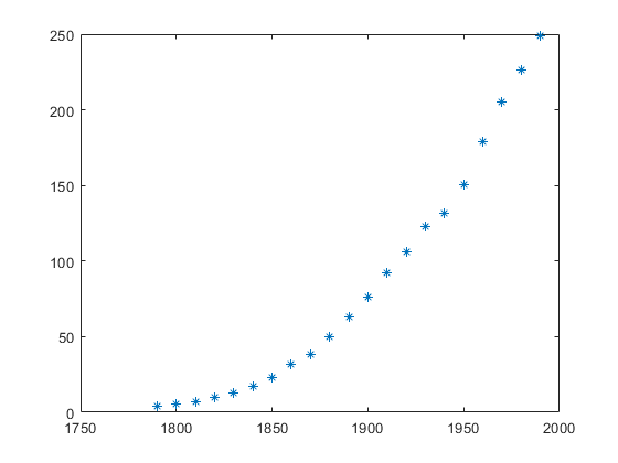
Census example

load census;
x = cdate;
y = pop;
plot(x, y, '*');

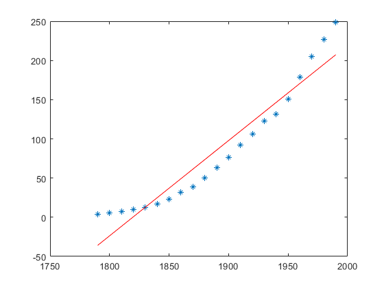
f = fit(x, y, 'poly1')

p = coeffvalues(f)

a = p(1)
b = p(2)

y_approx = a * x + b;

hold on;
plot(x, y_approx, 'r');

f = 

     Linear model Poly1:
     f(x) = p1*x + p2
     Coefficients (with 95% confidence bounds):
       p1 =       1.216  (1.045, 1.387)
       p2 =       -2212  (-2535, -1889)

p =

   1.0e+03 *

    0.0012   -2.2120


a =

    1.2157


b =

  -2.2120e+03

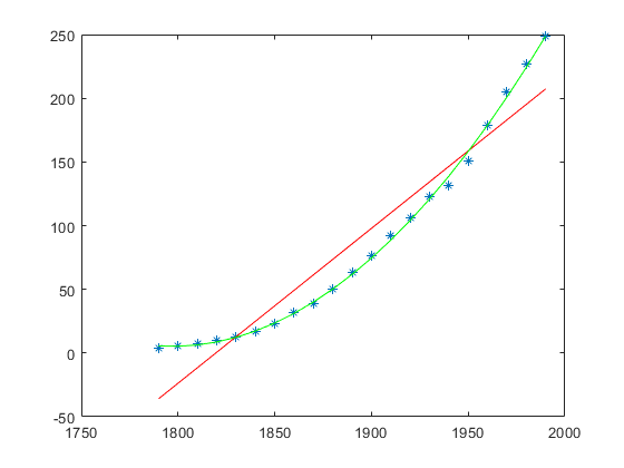
f = fit(x, y, 'poly2');

p = coeffvalues(f);

a = p(1);
b = p(2);
c = p(3);

y_approx_2 = a * x.^2 + b * x + c;
plot(x, y_approx_2, 'g');

LED

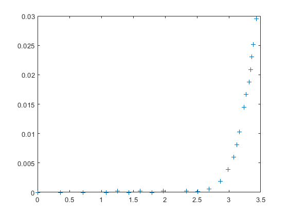
IV characteristic for an ideal LED is a sudden jump to \infty after the threshold voltage.

Measuring a real LED, we get values like these:

I_measured = [0, 0, 0, 0, 0.0002, 0, 0.0002, 0, 0.0002, 0.0002, 0.0001, ...
    0.0006, 0.00189, 0.00389, 0.00598, 0.00807, 0.01027, 0.01445, ...
    0.01664, 0.01874, 0.02083, 0.02302, 0.02512, 0.02950]';
V_measured = [0, 0.36091, 0.71343, 1.07434, 1.25060, 1.43525, 1.61151, ...
    1.79616, 1.97242, 2.33333, 2.50959, 2.68585, 2.87050, 2.98801, ...
    3.08034, 3.12230, 3.16427, 3.23981, 3.27338, 3.31535, 3.34053, ...
    3.35731, 3.38249, 3.43285]';

clf;
plot(V_measured, I_measured, '+');

Which we may try to fit with a single linear function:

f = fit(V_measured, I_measured, 'poly1');
p = coeffvalues(f);
a1 = p(1);
b1 = p(2);

I_predicted1 = a1 * V_measured + b1;

clf;
hold on;
plot(V_measured, I_measured, '+');
plot(V_measured, I_predicted1, 'r');

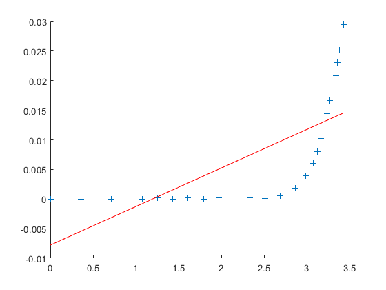
But this is very clearly a rather disappointing model.

Piecewise linear model

We may then attempt to model the IV curve by a set of linear pieces. The exercise mentions using 5 intervals, but not which data points each one covers, so we must decide that ourselves. After some attempts, the cleanest division I came across is:

num_intervals = 5;
points_per_interval = [11, 3, 3, 6, 5];

Which can then be converted to a list of "interval boundaries" with the following code. Reverse engineering not really relevant, it just adds them in a slightly special way to allow for a one point overlap

assert(length(points_per_interval) == num_intervals);
assert(sum(points_per_interval) - num_intervals + 1 == length(V_measured));

indices = [0 cumsum(points_per_interval)] + 1 - (0:5); %Voodoo magic

I_predicted2 = zeros([1, length(V_measured)]);

for i = 1 : 5
    i0 = indices(i);
    i1 = indices(i+1);

    V0 = V_measured(i0);
    V1 = V_measured(i1);

    f = fit(V_measured(i0:i1), I_measured(i0:i1), 'poly1');
    p = coeffvalues(f);
    a = p(1);
    b = p(2);

    I_predicted2(2*i-1) = a * V0 + b;
    I_predicted2(2*i) = a * V1 + b;

    plot([V0, V1], I_predicted2(2*i-1:2*i), 'g-');
end

x0, x1 = xlim;
y0, y1 = ylim;
for x = indices
    plot([x, x], [y0, y1], 'k--');
end
xlim([x0, x1]);
ylim([y0, y1]);

Unrecognized function or variable 'x0'.

Error in lab5 (line 128)
x0, x1 = xlim;