Lab 4, Ioan Dragomir

Intro

As seen in previous labs, most physical problems can be reduced to solving some ODE. Previously, we used Dsolve for this purpose, but another approach is using the odexy family of functions, which we will study in this lab. While dsolve would accept a system of differential equations and would figure out much of its structure by itself, ode23 and ode45 require a more targeted approach, where we categorically know which variables we will study over time, and whose derivatives we will need to calculate.

Van der Pol example

To illustrate the use of these ode solvers, we may use the Van der Pol oscillator as the system we want to simulate.

What we need to provide to ode23 is a function that describes the system in terms of first order derivatives, a time interval, and some initial conditions.

In our case, the function describing the Van der Pol oscillator is already a part of MATLAB and is called vdp1. It takes two input arguments: t, which is the current time, and in this case is unused, and y, which is a vector containing the current "state" of the circuit, boiled down to just two numbers. Its return value describes the derivative of those two values. In other words, the function calculates, for a given moment in time, how the oscillator is changing in that exact point in time. The ode23 function uses this function to "figure out" the behaviour of the signal over a larger period of time.

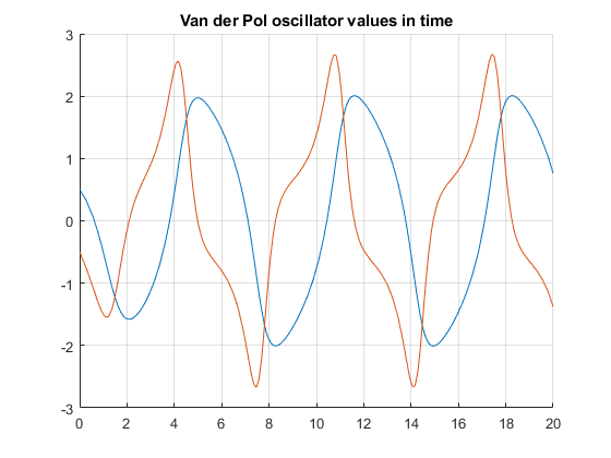
sim_time_interval = [0, 20];
sim_initial_conditions = [0.5, -0.5];

% Simulate!
sim_solution = ode23(@vdp1, sim_time_interval, sim_initial_conditions);

sim_times = sim_solution.x;   % Time values are not uniformly distributed,
                              % so we must explicitly extract them

sim_y1 = sim_solution.y(1,:); % First row of y
sim_y2 = sim_solution.y(2,:); % Second row of y

hold on;
plot(sim_times, sim_y1);
plot(sim_times, sim_y2);
grid();
title("Van der Pol oscillator values in time")
hold off;

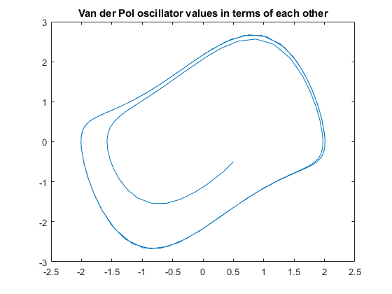
plot(sim_y1, sim_y2);
title("Van der Pol oscillator values in terms of each other")

Van der Pol in simulink

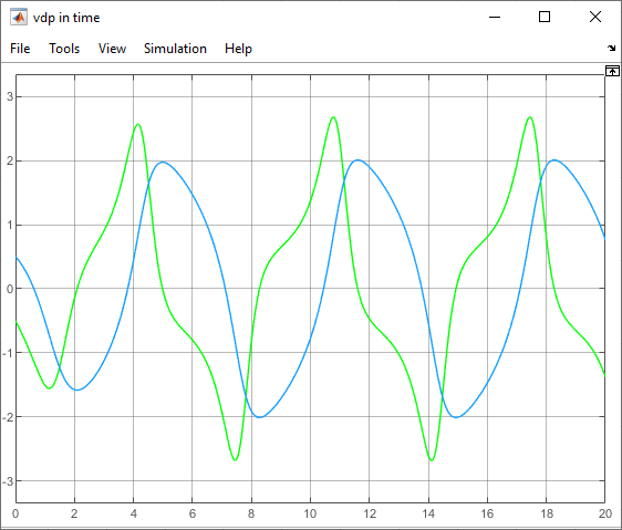
We may also build the Van der Pol function in simulink:

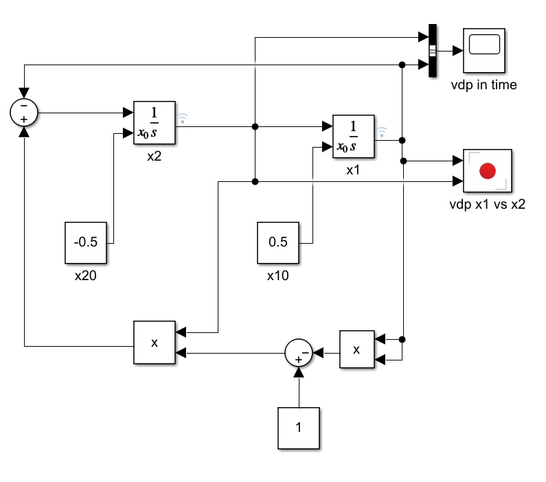
And we notice it produces the same results:

Download vdp_simulink.mdl

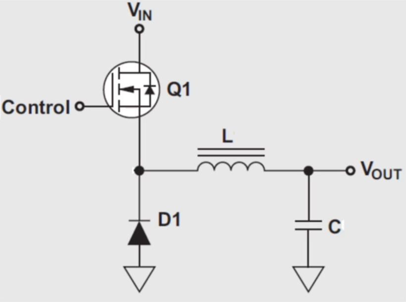
Buck (step-down) converter simulation

The buck converter is an usual circuit used to convert from a high voltage to a lower one. It functions by repeatedly switching a transistor on and off, which then feeds a filtering circuit:

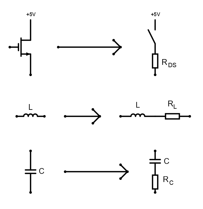
For a more correct simulation, we will use non-ideal models of the transistor, inductor and capacitor:

Also, we will add a resistance \(R_{ld}\) to simulate the equivalent resistance of the circuit powered by this converter. If it weren't for this, the energy we intend to convert wouldn't be used anywhere and the system would just quickly charge up and stay static.

The whole circuit now looks like this:

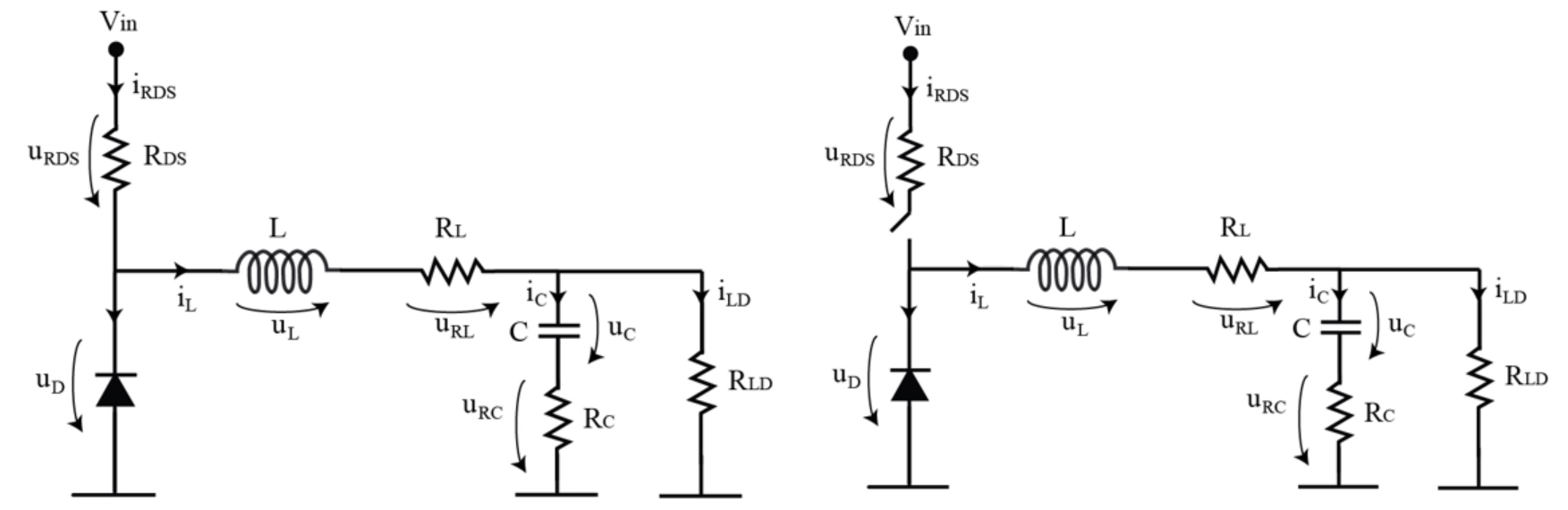
There are two variants, one with the switch kept open and one closed, to describe the equivalent circuit when the transistor is on versus off.

I will add the simulation parameters here so the following code works without symbolic variables. These values are only introduced in exercise 2.

global V_in V_D;

R_ld = 2.5;    % (ohm)
R_DS = 0.02;   % (ohm)
R_L = 0.037;   % (ohm)
L = 12e-6;     % (12uH)
R_C = 0.025;   % (ohm)
C = 4e-6;      % (4uF)
V_in = 12;     % (V)
V_D = 0.4;     % (V)
F_sw = 400000; % 400KHz switching frequency
D = 0.42;      % 42% ducty cycle

Exercise 1 - state choice, state-space realization matrix

We now need to choose which variables we want to simulate through time, our state variables. A good choice is \(i_L\) and \(u_C\), from two different standpoints:

On the one hand, mathematically, we have clean formulas that describe the derivatives of the current through an inductor (\(i_L' = v/L\)) and the voltage across a capacitor (\(v_C' = i/C\)).

On the other hand, as mentioned in the lab material, the inductor and capacitor are the only two elements that actually "store" energy and, in a way, influence the circuit as a whole over time. The current through or voltage across one of the resistors, for example, physically tells us much less than the two chosen variables.

To be able to use our ODE solver functions, we need to express the derivatives of \(i_L\) and \(v_C\) in terms of the two variables themselves, as well as the simulation parameters.

For the first excercise, we need to write these two formulas in matrix form. That is, find some \(A, B, C, D, E, F\) such that:

\[ \begin{pmatrix} A & B \\ C & D \end{pmatrix} \cdot \begin{pmatrix} i_L \\ u_C \end{pmatrix} + \begin{pmatrix} E \\ F \end{pmatrix} V_{in} = \begin{pmatrix} \frac{di_L}{dt} \\ \frac{du_C}{dt} \end{pmatrix} \]

ON state

Initially, we will study the ON state.

It took me a lot of trial and error, but I finally arrived at the result through this process. First, we write the output voltage in terms of the capacitor branch's values.

\[ V_{out} = u_C + i_C R_C = u_C + \frac{du_C}{dt}CR_C \]

so that we may write \(i_{ld}\) in two different ways to eliminate it from the equation. In all my tries, \(i_{ld}\) was the hardest object to eliminate from the equations.

\[ \begin{aligned} i_{ld} &= V_{out} / R_{ld} = \frac{u_C + \frac{du_C}{dt}CR_C}{R_{ld}} \\ i_{ld} &= i_L - i_C = i_L - C\frac{du_C}{dt} \end{aligned} \]

These two can be rearranged to obtain just \(du_C/dt\):

\[ \begin{aligned} &\frac{u_C + \frac{du_C}{dt}CR_C}{R_{ld}} = i_L - C\frac{du_C}{dt} \\ &\frac{du_C}{dt}(CR_C + CR_{ld}) = R_{ld}i_L - u_C \\ &\frac{du_C}{dt} = \frac{1}{C}\frac{R_{ld}i_L - u_C}{R_C + R_{ld}} \end{aligned} \]

We notice the last formula is entirely composed of parameters and state variables, so it is in the form we need. We now need to find an expression for \(i_L\). For this, we start by applying KVL on the \(V_{in} - L - C - 0\) path:

\[ V_{in} = i_L R_{DS} + u_L + i_L R_L + u_C + i_C R_C \]

Then we plug in the inductor and capacitor formulas:

\[ V_{in} = i_L R_{DS} + L\frac{di_L}{dt} + i_L R_L + u_C + C\frac{du_C}{dt} R_C \]

And use the previous result for \(du_C/dt\):

\[ V_{in} = i_L R_{DS} + L\frac{di_L}{dt} + i_L R_L + u_C + \frac{R_{ld}i_L - u_C}{R_C + R_{ld}} R_C \]

From the last step, we already have \(du_C/dt\), so we can see all terms are known values, from which we can extract \(di_L/dt\):

\[ \frac{di_L}{dt} = \frac{1}{L}\left( V_{in} - i_L R_{DS} - i_L R_L - u_C - \frac{R_{ld}i_L - u_C}{R_C + R_{ld}} R_C \right) \]

To get to the wanted matrix form, we need to "factor out" \(i_L\) and \(u_C\) from the formulas we have:

\[ \begin{aligned} \frac{di_L}{dt} &= \frac{1}{L}\left( V_{in} - i_L R_{DS} - i_L R_L - u_C - \frac{R_{ld}i_L - u_C}{R_C + R_{ld}} R_C \right) \\ &= i_L \cdot -\frac{1}{L} (R_{DS} + R_L + \frac{R_C}{R_C + R_{ld}}) + u_C \cdot -\frac{1}{L} (1 - \frac{R_C}{R_C + R_{ld}}) + \frac{V_{in}}{L} \\ \frac{du_C}{dt} &= \frac{1}{C}\frac{R_{ld}i_L - u_C}{R_C + R_{ld}} \\ &= i_L \cdot \frac{R_ld}{C(R_C + R_{ld})} + u_C \cdot \frac{-1}{C(R_C + R_{ld})} \end{aligned} \]

Thus we can write:

\[ \begin{pmatrix} \frac{di_L}{dt} \\ \frac{du_C}{dt} \end{pmatrix} = \begin{pmatrix} -\frac{1}{L} (R_{DS} + R_L + \frac{R_C}{R_C + R_{ld}}) & -\frac{1}{L} (1 - \frac{R_C}{R_C + R_{ld}}) \\ \frac{R_{ld}}{C(R_C + R_{ld})} & \frac{-1}{C(R_C + R_{ld})} \end{pmatrix} \cdot \begin{pmatrix} i_L \\ u_C \end{pmatrix} + \begin{pmatrix} \frac{1}{L} \\ 0 \end{pmatrix} \cdot V_{in} \]

global buck_on_A buck_on_B;

buck_on_A = [
    -(R_DS + R_L + R_C/(R_C + R_ld))/L,   -(1 - R_C/(R_C + R_ld))/L;
    R_ld/(C*(R_C + R_ld)),                -1/(C*(R_C + R_ld))
];
buck_on_B = [1/L; 0];

OFF state

For the off state, the formulas are very similar, but we do not have the influence of \(V_{in}\) and \(R_{DS}\), and instead have our input voltage determined by the diode, with voltage \(V_D\).

Intuitively, this is due to the fact that the circuit as a whole is largely unchanged, and the relationships between the inductor and capacitor are the same regardless whether the input energy comes from \(V_{in}\) or \(V_D\). We may mentally separate everything to the left of the inductor to an imaginary "energy source" element.

\[ \begin{pmatrix} \frac{di_L}{dt} \\ \frac{du_C}{dt} \end{pmatrix} = \begin{pmatrix} -\frac{1}{L} (R_L + \frac{R_C}{R_C + R_{ld}}) & -\frac{1}{L} (1 - \frac{R_C}{R_C + R_{ld}}) \\ \frac{R_{ld}}{C(R_C + R_{ld})} & \frac{-1}{C(R_C + R_{ld})} \end{pmatrix} \cdot \begin{pmatrix} i_L \\ u_C \end{pmatrix} + \begin{pmatrix} \frac{1}{L} \\ 0 \end{pmatrix} \cdot V_D \]

global buck_off_A buck_off_B;

buck_off_A = [
    -(R_L + R_C/(R_C + R_ld))/L,   -(1 - R_C/(R_C + R_ld))/L;
    R_ld/(C*(R_C + R_ld)),         -1/(C*(R_C + R_ld))
];

buck_off_B = [1/L; 0];

Excercise 2 - writing ode functions

As mentioned before, our functions need to take input arguments of the form (t, state_vector) and return the derivatives of the elements in the state vector. In our case, we do this by matrix multiplication, but the computation can be done in any way we want. There are other forms in which it would have been considerably easier to read...

function derivs = buck_on(t, x)
    global buck_on_A buck_on_B V_in;
    derivs = buck_on_A * x + buck_on_B * V_in;
end

function derivs = buck_off(t, x)
    global buck_off_A buck_off_B V_D;
    derivs = buck_off_A * x + buck_off_B * V_D;
end

Excercise 3 - simulating the buck converter

For this excercise, we need to bring everything we just did together and actually simulate the circuit from time 0 to 1ms.

For easier computations, we may define some time constants that describe the time period of an on-off cycle, as well as how long the on part takes:

T = 1 / F_sw;
T_on = T * D;

Initially, \((i_L\ u_C)^t = (0\ 0)^t\):

state = [0; 0];

Now, to actually simulate the system, we will do it in time slices. There will be a period of the system behaving as buck_on, then a period as buck_off, repeat. When passing from one period to the next, we will need to "maintain" the system state, so it doesn't reset to some initial default.

We will declare some arrays to keep track of all the simulated states over time, so we can plot them later:

sim_times = [];
sim_states = [];

Now, for each period of duration \(T\) from 0 to 1ms:

for t = 0 : T : 1e-3

We will use ode45 to simulate the behaviour defined by buck_on, from time t to time t+T_on, with initial conditions given by the state variable:

    [sim_on_times, sim_on_states] = ode45(@buck_on, [t, t+T_on], state);

The return value is a pair of a vector containing times and a vector containing the states at each of those times. To simulate our system further, we need to extract these two, and also find the last state:

    state = sim_on_states(end,:);

Then we pass it to another call of ode45, which is very similar to the last one, but now simulates on the time interval t+T_on to t+T and starts from the new state:

    [sim_off_times, sim_off_states] = ode45(@buck_off, [t+T_on, t+T], state);

    state = sim_off_states(end,:);

At the end of each time slice, we append the time and state data we just simulated in this time slice to the list of all time and state data points:

    sim_times = [sim_times ; sim_on_times ; sim_off_times];
    sim_states = [sim_states ; sim_on_states ; sim_off_states];

end

Finally, we draw a plot of all the data points. On the x axis we have the times specified by sim_times and on the y axis we have the pairs of \(i_L\) and \(u_C\) values in each row of sim_states:

plot(sim_times, sim_states);
legend(["iL", "uC"]);
title("Buck converter simulation");

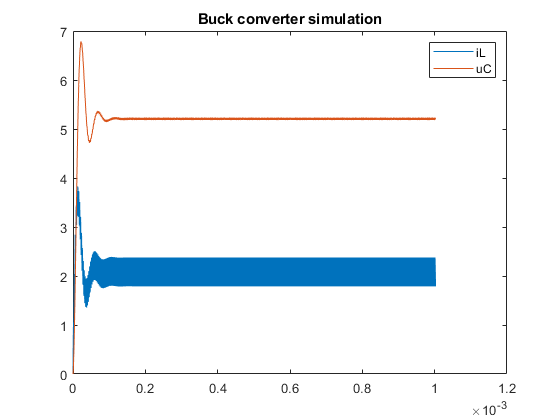
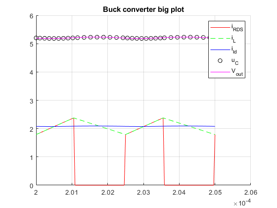
As requested by the exercise, we will also plot the current through the switch \(i_{RDS}\), the current through the inductor \(i_L\), the voltage drop across the capacitor \(u_C\), the output voltage \(V_{out}\), and the load current \(i_{ld}\), during 2 periods in the static regime. That is, an on-off-on-off cycle after the circuit stabilizes, which we can see from the previous graph happens after around 0.15ms; we'll say 0.2ms to be safe.

t0 = 0.2 * 10^-3;
t1 = t0 + 2*T;

Because the data points we have are not evenly spaced apart in time, we will have to deal with a little bit of trouble of differentiating between times and indices in our simulation data. To start, we will find some indices that roughly delimit the time period we're interested in:

it0 = find(sim_times >= t0, 1);
it1 = find(sim_times >= t1, 1);

And then select the time and state data between those indices:

times = sim_times(it0:it1);
i_L = sim_states(it0:it1, 1);
u_C = sim_states(it0:it1, 2);

Now, using formulas we have previously explored, we obtain the other circuit variables in terms of the parameters and \(i_L\) and \(u_C\):

\[ \begin{aligned} V_{out} &= u_C + u_{RC} \\ &= u_C + R_C i_C \\ &= u_C + R_C C \frac{du_C}{dt} \\ &= u_C + R_C C \frac{1}{C}\frac{R_{ld}i_L - u_C}{R_C + R_{ld}} \\ &= u_C + R_C \frac{R_{ld}i_L - u_C}{R_C + R_{ld}} \end{aligned} \]

V_out = u_C + R_C * (R_ld * i_L - u_C)/ (R_C + R_ld);

\[ i_{ld} = \frac{V_{out}}{R_{ld}} \]

i_ld = V_out / R_ld;

For \(i_{RDS}\) we don't have a perfectly clean formula in terms of the state variables, because it is, in a way, one of the inputs themselves. We iterate through all data points from time t0 to t1. That is, all points from index it0 to it1:

i_RDS = zeros([it1 - it0 + 1, 1]);
for i = it0 : it1

    % For each index, we get the corresponding time
    t = sim_times(i);

and if it falls in the ON part of the period, we have \(i_{RDS} = i_L\). Otherwise it is zero.

    if mod(t, T) <= T_on
        i_RDS(i - it0 + 1) = sim_states(i, 1);
    else
        i_RDS(i - it0 + 1) = 0;
    end

end

Finally, we can plot all these variables:

clf;
hold on;
title("Buck converter big plot");
plot(times, i_RDS, "r-");
plot(times, i_L, "g--");
plot(times, i_ld, "b");
plot(times(1:5:end), u_C(1:5:end), "ko");
plot(times, V_out, "m-");
grid();
legend(["i_{RDS}", "i_L", "i_{ld}", "u_C", "V_{out}"]);

... Here are the buck_on and buck_off functions.

function derivs = buck_on(t, x)
    global buck_on_A buck_on_B V_in;
    derivs = buck_on_A * x + buck_on_B * V_in;
end

function derivs = buck_off(t, x)
    global buck_off_A buck_off_B V_D;
    derivs = buck_off_A * x + buck_off_B * V_D;
end

Download me!

You can download this by just running the MATLAB command:

grabcode("https://trupples.space/uni/2/ProcessModeling/html/lab4.html")

Or by clicking: download lab4.m